Automatic Hyperparameter Tuning
In this notebook we show how the franken library can be used to automatically find the best hyperparameters (HPs) for fitting potential functions on a given dataset. The HP search procedure is a simple grid-search over
The kernel parameters (e.g length-scale, polynomial degree, …)
The solver parameters (e.g. force-weight, ridge penalty, …)
This tuning procedure can be equivalently run using the code from this notebook, or from the command-line using the franken.autotune command and specifying all options on the CLI.
This notebook is also available on Google colab for easy running.
[1]:
try:
    import franken
except ImportError:
    %pip install franken[mace]
    import franken
[2]:
import json

import matplotlib
import matplotlib.pyplot as plt
import pandas as pd

from franken.autotune import autotune
from franken.config import MaceBackboneConfig, GaussianRFConfig, DatasetConfig, SolverConfig, HPSearchConfig, AutotuneConfig
/home/lbonati@iit.local/software/miniforge3-mamba/envs/franken/lib/python3.13/site-packages/tqdm/auto.py:21: TqdmWarning: IProgress not found. Please update jupyter and ipywidgets. See https://ipywidgets.readthedocs.io/en/stable/user_install.html
  from .autonotebook import tqdm as notebook_tqdm
The process of running autotune is simple: first initialize all configuration objects. These will also include the definition of the hyperparameter search-space. Then simply pass all objects to autotune which will run the training algorithm for each hyperparameters setting and figure out which one performs the best. For this to work it is very important to provide a validation dataset which is different from the training set. The “water” dataset we use in the notebook also comes with
a pre-defined validation split.
[3]:
from franken.datasets.registry import DATASET_REGISTRY
from franken.backbones.utils import CacheDir

train_path = DATASET_REGISTRY.get_path("water", "train", base_path=CacheDir.get())
val_path = DATASET_REGISTRY.get_path("water", "val", base_path=CacheDir.get())

print(f"Train path: {train_path}")
print(f"Val path: {val_path}")
Train path: /home/lbonati@iit.local/.franken/water/ML_AB_dataset_1.xyz
Val path: /home/lbonati@iit.local/.franken/water/ML_AB_dataset_2-val.xyz
The equivalent franken.autotune command to the configuration defined here is:
franken.autotune \
    --train-path $HOME/.franken/water/ML_AB_dataset_1.xyz
    --val-path $HOME/.franken/water/ML_AB_dataset_2-val.xyz
    --max-train-samples 8 \
    --l2-penalty="(-10, -5, 5, log)" \
    --force-weight="(0.01, 0.99, 5, linear)" \
    --metrics energy_MAE forces_MAE \
    --seed 42 \
    --jac-chunk-size "auto" \
    --run-dir "./results" \
    --backbone=mace --mace.path-or-id "mace_mp/small" --mace.interaction-block 2 \
    --rf=gaussian --gaussian.num-rf 512 --gaussian.length-scale="[1., 5., 10.0, 15.0, 20.0, 25.0, 30.0]"
The GNN and dataset configurations are fixed. We use just 8 training samples to reduce the computation time for CoLab, but if you run this locally you can increase it.
[4]:
gnn_config = MaceBackboneConfig(
    path_or_id="mace_mp/small",
    interaction_block=2,
)
dataset_cfg = DatasetConfig(train_path=str(train_path),
                            max_train_samples=8,
                            val_path=str(val_path)
)
We use Gaussian random features to run the automatic tuning on the length-scale parameter. autotune will test some values from 1 to 30.
[5]:
rf_config = GaussianRFConfig(
    num_random_features=512,
    length_scale=HPSearchConfig(values=[1., 5., 10.0, 15.0, 20.0, 25.0, 30.0]),
    rng_seed=42,  # for reproducibility
)
The solver parameters are less expensive to iterate over, so we can use a finer grid. For the l2_penalty HP we will test 5 logarithmically-spaced values between \(10^{-10}\) and \(10^{-5}\), and for the force_weight HP we will test 5 linearly-spaced values between 0.01 and 0.99.
[6]:
solver_cfg = SolverConfig(
    l2_penalty=HPSearchConfig(start=-10, stop=-5, num=5, scale='log'),  # equivalent of numpy.logspace
    force_weight=HPSearchConfig(start=0.01, stop=0.99, num=5, scale='linear'),  # equivalent of numpy.linspace
)
Finally all configurations are grouped together and we run autotune. Note the run_dir setting: this is where the logs and models will be saved.
[7]:
autotune_cfg = AutotuneConfig(
    dataset=dataset_cfg,
    solver=solver_cfg,
    backbone=gnn_config,
    rfs=rf_config,
    metrics=["energy_MAE", "forces_MAE"],
    seed=42,
    jac_chunk_size='auto',
    run_dir="./results",
)

run_path = autotune(autotune_cfg)
console_logging_level: INFO
dtype: float64
jac_chunk_size: auto
rf_normalization: leading_eig
run_dir: ./results
save_every_model: False
save_fmaps: False
scale_by_species: True
seed: 42
backbone:
    family: mace
    interaction_block: 2
    path_or_id: mace_mp/small
dataset:
    max_train_samples: 8
    name: null
    test_path: null
    train_path: /home/lbonati@iit.local/.franken/water/ML_AB_dataset_1.xyz
    val_path: /home/lbonati@iit.local/.franken/water/ML_AB_dataset_2-val.xyz
metrics:
    - energy_MAE
    - forces_MAE
rfs:
    length_scale:
      num: null
      scale: null
      start: null
      stop: null
      value: null
      values:
      - 1.0
      - 5.0
      - 10.0
      - 15.0
      - 20.0
      - 25.0
      - 30.0
    num_random_features: 512
    rf_type: gaussian
    rng_seed: 42
    use_offset: true
solver:
    force_weight:
      num: 5
      scale: linear
      start: 0.01
      stop: 0.99
      value: null
      values: null
    l2_penalty:
      num: 5
      scale: log
      start: -10
      stop: -5
      value: null
      values: null

2026-02-10 16:15:03.521 WARNING (rank 0): Cache directory already initialized at /home/lbonati@iit.local/.franken. Reinitializing.
2026-02-10 16:15:03.522 INFO (rank 0): Initializing default cache directory at /home/lbonati@iit.local/.franken
2026-02-10 16:15:03.545 INFO (rank 0): Run folder: results/run_260210_161503_ecf01a5f
cuequivariance or cuequivariance_torch is not available. Cuequivariance acceleration will be disabled.
ASE -> MACE (train): 100%|██████████| 8/8 [00:00<00:00, 145.20it/s]
ASE -> MACE (val): 100%|██████████| 189/189 [00:00<00:00, 248.05it/s]
Computing dataset statistics: 100%|██████████| 8/8 [00:00<00:00, 17.58it/s]
2026-02-10 16:15:12.382 INFO (rank 0): jacobian chunk size automatically set to 32
2026-02-10 16:15:44.109 WARNING (rank 0): `leading_eig` normalization has high memory usage. If you encounter OOM errors try to disable it.
2026-02-10 16:16:29.210 INFO (rank 0): Trial   1 | rf_type: gaussian | num_random_features:   512   | length_scale:  1.000  | use_offset:  True   | rng_seed:   42    | Best trial 1 (energy 1.48 meV/atom - forces 96.7 meV/Ang)
2026-02-10 16:16:34.821 INFO (rank 0): jacobian chunk size automatically set to 32
2026-02-10 16:17:05.039 WARNING (rank 0): `leading_eig` normalization has high memory usage. If you encounter OOM errors try to disable it.
2026-02-10 16:17:49.492 INFO (rank 0): Trial   2 | rf_type: gaussian | num_random_features:   512   | length_scale:  5.000  | use_offset:  True   | rng_seed:   42    | Best trial 2 (energy 0.38 meV/atom - forces 28.1 meV/Ang)
2026-02-10 16:17:54.961 INFO (rank 0): jacobian chunk size automatically set to 32
2026-02-10 16:18:25.419 WARNING (rank 0): `leading_eig` normalization has high memory usage. If you encounter OOM errors try to disable it.
2026-02-10 16:19:10.188 INFO (rank 0): Trial   3 | rf_type: gaussian | num_random_features:   512   | length_scale: 10.000  | use_offset:  True   | rng_seed:   42    | Best trial 3 (energy 0.34 meV/atom - forces 25.9 meV/Ang)
2026-02-10 16:19:15.820 INFO (rank 0): jacobian chunk size automatically set to 32
2026-02-10 16:19:48.589 WARNING (rank 0): `leading_eig` normalization has high memory usage. If you encounter OOM errors try to disable it.
2026-02-10 16:20:35.754 INFO (rank 0): Trial   4 | rf_type: gaussian | num_random_features:   512   | length_scale: 15.000  | use_offset:  True   | rng_seed:   42    | Best trial 4 (energy 0.32 meV/atom - forces 25.3 meV/Ang)
2026-02-10 16:20:41.424 INFO (rank 0): jacobian chunk size automatically set to 32
2026-02-10 16:21:13.832 WARNING (rank 0): `leading_eig` normalization has high memory usage. If you encounter OOM errors try to disable it.
2026-02-10 16:21:58.791 INFO (rank 0): Trial   5 | rf_type: gaussian | num_random_features:   512   | length_scale: 20.000  | use_offset:  True   | rng_seed:   42    | Best trial 5 (energy 0.34 meV/atom - forces 25.0 meV/Ang)
2026-02-10 16:22:04.323 INFO (rank 0): jacobian chunk size automatically set to 32
2026-02-10 16:22:34.677 WARNING (rank 0): `leading_eig` normalization has high memory usage. If you encounter OOM errors try to disable it.
2026-02-10 16:23:20.463 INFO (rank 0): Trial   6 | rf_type: gaussian | num_random_features:   512   | length_scale: 25.000  | use_offset:  True   | rng_seed:   42    | Best trial 6 (energy 0.33 meV/atom - forces 24.8 meV/Ang)
2026-02-10 16:23:26.247 INFO (rank 0): jacobian chunk size automatically set to 32
2026-02-10 16:23:58.504 WARNING (rank 0): `leading_eig` normalization has high memory usage. If you encounter OOM errors try to disable it.
2026-02-10 16:24:45.309 INFO (rank 0): Trial   7 | rf_type: gaussian | num_random_features:   512   | length_scale: 30.000  | use_offset:  True   | rng_seed:   42    | Best trial 7 (energy 0.32 meV/atom - forces 24.6 meV/Ang)
Analysing the results
There are two main outputs from the autotune procedure: the model trained with the best hyperparameters, which is saved at "results/best_ckpt.pt" and the logs which describe the errors of all the models trained. Here we analyze the error-log, and in the molecular_dynamics notebook we will use the trained model to perform some MD simulations.
[8]:
# We load the full logs for all training runs and the logs for just the best model.
with open(run_path / "log.json", "r") as fh:
    all_logs = json.load(fh)
with open(run_path / "best.json", "r") as fh:
    best_log = json.load(fh)
[9]:
best_ls = best_log["hyperparameters"]["random_features"]["length_scale"]
best_l2 = best_log["hyperparameters"]["solver"]["l2_penalty"]
best_fw = best_log["hyperparameters"]["solver"]["force_weight"]
print("Best hyperparameters: ")
print(f"\tLength-scale: {best_ls:.1f}")
print(f"\tL2 penalty: {best_l2:.2e}")
print(f"\tForce-weight: {best_fw:.3f}")
Best hyperparameters:
        Length-scale: 30.0
        L2 penalty: 1.78e-09
        Force-weight: 0.010
To make the analysis easier we convert the json logs to pandas
[10]:
logs_df = pd.json_normalize(all_logs)  # flattens nested dictionaries and converts to DataFrame
logs_df.head()
[10]:
| checkpoint.hash | checkpoint.rf_weight_id | timings.cov_coeffs | timings.solve | metrics.train.energy_MAE | metrics.train.forces_MAE | metrics.validation.energy_MAE | metrics.validation.forces_MAE | hyperparameters.franken.path_or_id | hyperparameters.franken.interaction_block | hyperparameters.franken.family | hyperparameters.random_features.rf_type | hyperparameters.random_features.num_random_features | hyperparameters.random_features.length_scale | hyperparameters.random_features.use_offset | hyperparameters.random_features.rng_seed | hyperparameters.input_scaler.scale_by_Z | hyperparameters.solver.force_weight | hyperparameters.solver.l2_penalty | hyperparameters.solver.dtype | |
|---|---|---|---|---|---|---|---|---|---|---|---|---|---|---|---|---|---|---|---|---|
| 0 | 1566c4e8d00298883c7def9b5e59e352 | 0 | 37.597101 | 0.005464 | 0.038367 | 63.922082 | 1.217128 | 97.950285 | mace_mp/small | 2 | mace | gaussian | 512 | 1.0 | True | 42 | True | 0.01 | 1.000000e-10 | torch.float64 |
| 1 | 1566c4e8d00298883c7def9b5e59e352 | 1 | 37.597101 | 0.001383 | 0.038376 | 63.921710 | 1.217229 | 97.946695 | mace_mp/small | 2 | mace | gaussian | 512 | 1.0 | True | 42 | True | 0.01 | 1.778279e-09 | torch.float64 |
| 2 | 1566c4e8d00298883c7def9b5e59e352 | 2 | 37.597101 | 0.001512 | 0.038521 | 63.916007 | 1.219013 | 97.884128 | mace_mp/small | 2 | mace | gaussian | 512 | 1.0 | True | 42 | True | 0.01 | 3.162278e-08 | torch.float64 |
| 3 | 1566c4e8d00298883c7def9b5e59e352 | 3 | 37.597101 | 0.001474 | 0.041016 | 63.985303 | 1.246055 | 97.092725 | mace_mp/small | 2 | mace | gaussian | 512 | 1.0 | True | 42 | True | 0.01 | 5.623413e-07 | torch.float64 |
| 4 | 1566c4e8d00298883c7def9b5e59e352 | 4 | 37.597101 | 0.001303 | 0.063570 | 70.761652 | 1.362110 | 98.960269 | mace_mp/small | 2 | mace | gaussian | 512 | 1.0 | True | 42 | True | 0.01 | 1.000000e-05 | torch.float64 |
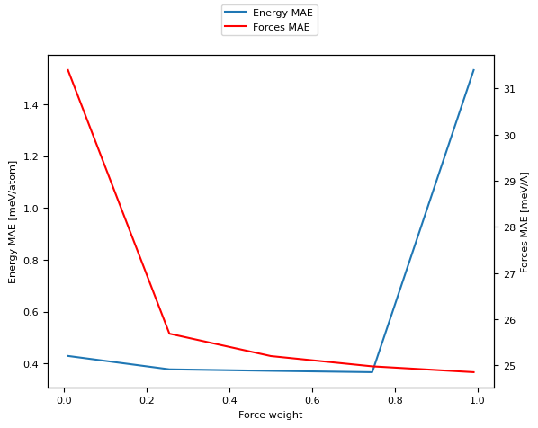
Since we have three different hyperparameters it’s hard to visualize their behavior all at the same time. We start by analyzing the behavior as the forces-weight changes from very low to very high, plotting the error on both forces and energy predictions.
[11]:
df_fw = logs_df[  # Fix the other two hyperparameters
    (logs_df["hyperparameters.random_features.length_scale"] == best_ls) &
    ((logs_df["hyperparameters.solver.l2_penalty"] - 5.62341325e-07).abs() < 1e-12)
]
df_fw = df_fw.sort_values("hyperparameters.solver.force_weight")
fig, ax = plt.subplots()
ax.plot(
    df_fw["hyperparameters.solver.force_weight"],
    df_fw["metrics.validation.energy_MAE"],
    label="Energy MAE"
)
ax2 = ax.twinx()
ax2.plot(
    df_fw["hyperparameters.solver.force_weight"],
    df_fw["metrics.validation.forces_MAE"],
    label="Forces MAE",
    c='r'
)
fig.legend(loc='upper center')
ax.set_xlabel("Force weight")
ax.set_ylabel("Energy MAE [meV/atom]")
ax2.set_ylabel("Forces MAE [meV/A]")
[11]:
Text(0, 0.5, 'Forces MAE [meV/A]')
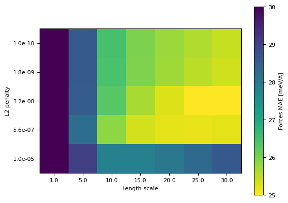
Next we analyze the behaviour of the length-scale and l2 penalty hyperparameters
[12]:
df_ker = logs_df[logs_df["hyperparameters.solver.force_weight"] == 0.5]
fig, ax = plt.subplots()
pivot = df_ker.pivot_table(
    index="hyperparameters.solver.l2_penalty",
    columns="hyperparameters.random_features.length_scale",
    values="metrics.validation.forces_MAE"
)
im = ax.imshow(pivot, norm=matplotlib.colors.Normalize(vmin=25, vmax=30), cmap="viridis_r")
cb = fig.colorbar(im)
cb.set_label("Forces MAE [meV/A]")
ax.set_xticks(range(len(pivot.columns)), pivot.columns)
ax.set_xlabel("Length-scale")
ax.set_yticks(range(len(pivot.index)), [f"{i:.1e}" for i in pivot.index])
ax.set_ylabel("L2 penalty")
[12]:
Text(0, 0.5, 'L2 penalty')